Micro 4/3

Micro 4/3 is the camera/sensor format I generally use for photomacrography. My present (as of 2023) Micro 4/3 camera I use in photomacrography and for most general photography is the OM System OM-1. The 4/3 in the name indicates the aspect ratio of the image. Do not confuse it with absolute sizes of sensors like 1/2" or 2/3". However, the Micro 4/3 sensor size also happens to fit the old 4/3" Vidicon size specification, which, confusingly, is much smaller than 4/3 of an inch.

4/3 was an Olympus DSLR format. Micro 4/3 is exactly the same sensor format and aspect ratio, but in a mirrorless camera. 4/3 and Micro 4/3 therefore use different lens mounts.

There are a few dedicated videocameras with Micro 4/3 lens mounts, but often their sensors are not the same physical size and aspect ratio as those of Micro 4/3 mirrorless cameras.

On this page, I list or compute the most frequently used parameters of the sensor in my OM-1, to help myself, and potentially others using Micro 4/3 cameras, when looking for these frequently-used parameters to plug into my calculations. For the data I did not measure myself, I report a link to an Internet source of these measurements.

Sensor size

The physical size of a Micro 4/3 sensor is around 18 mm × 13.5 mm (22.5 mm diagonal), according to Wikipedia. It is entirely possible that the substrate of sensors in different Micro 4/3 cameras is of slightly different sizes. These differences normally do not affect the active sensor area (i.e. the area covered by used pixels), only the margins between the edge of the active area and the physical edge of the chip substrate. It is also common for strips of non-active pixels, a few pixels wide, to be present around the area occupied by active pixels.

The active area of the OM-1 sensor, used to record images, is 17.4mm x 13mm according to DPReview, or 17.3 mm × 13.0 mm (21.6 mm diagonal) for any Micro 4/3 sensor, according to Wikipedia. However, according to other sources this second size seems to apply only to Panasonic Micro 4/3 cameras.

Neither figure seems to be accurate, because calculating the pixel pitch (which potentially includes any empty margin around a pixel) with either horizontal size divided by the horizontal pixel count (see below) gives:

17.4 / 5184 = 0.003357 mm
17.3 / 5184 = 0.003337 mm

But the vertical pixel pitch is instead:

13 / 3888 = 0.003343 mm

Since the pixels are square, the vertical and horizontal pixel pitch should be the same. The difference is small, but it is at the third significant digit and can make a difference in calculations, making the results slightly inconsistent. If we average the two horizontal pixel pitches we obtain

(0.003357+ 0.003337) / 2 = 0.003347 mm

This last figure is actually closer to the vertical pixel pitch than either "official" figure. Therefore, I decided to use in my calculations 17.35 x 13 mm (diagonal 21.7 mm) as the actual size of the active area, and 3.347 μm (4.731 μm diagonal) as the pixel pitch.

Pixel count

The "official" pixel count of Micro 4/3 sensors used in top-of-the-line Micro 4/3 cameras by Olympus and OM System is 20 Mpixels (the legacy EM-1 "Mark 1" has 16 Mpixels).

The active area (i.e. the area covered by active pixels, used to record images) is 5,184 (horizontal) x 3,888 (vertical) pixels. This is the size in pixels of an image recorded at native sensor resolution in single-exposure mode, at the maximum in-camera configurable resolution, without sensor-shift resolution-enhancement modes. The Olympus E-M1X, E-M1 III and E-M1 II also have the same sensor active area. Aside from this, the sensor of the OM-1 differs in several respects from those of earlier cameras.

Calculating from the number of pixels in an image saved on the OM-1, the number of active pixels is 5,184 * 3,888 = 20,155,392.

Nyquist limit

The Nyquist limit is the minimum spacing of line pairs that still allows each line to be distinguished. This limit is one cycle, i.e. two pixels, since each line, at a minimum, is one pixel thick.

Since diagonal pixel pitch is larger than horizontal and vertical pixel pitch, diagonal lines must be spaced further apart to still be rendered as distinct lines.

One difficulty is that the closest possible line pairs inclined at 45° are rendered as a checkerboard pattern by sampling algorithms that enhance fine-scale detail, or as a uniform blur by algorithms that suppress it, so in either case one cannot distinguish in which direction the lines are actually tilted. This phenomenon is closely related to aliasing. Nonetheless, I decided to use the same definition (one cycle) even in this worst-case situation.

The Nyquist limit expressed in length units is therefore 6.694 μm (9.461 μm diagonal).

A few sources on the Internet state that, for imaging applications, one should set the Nyquist limit slightly higher than one cycle. A limit of 1.35 cycles has been stated at least once. There are also assertions that other applications, like NIR imaging, require an even higher number of cycles. I did not find mathematical/physical explanations for this, and it seems to be a rule-of-thumb, more than a precise criterion. The large majority of sources only mention a limit of one cycle, which is the original definition by Nyquist. The latter is the convention I follow here.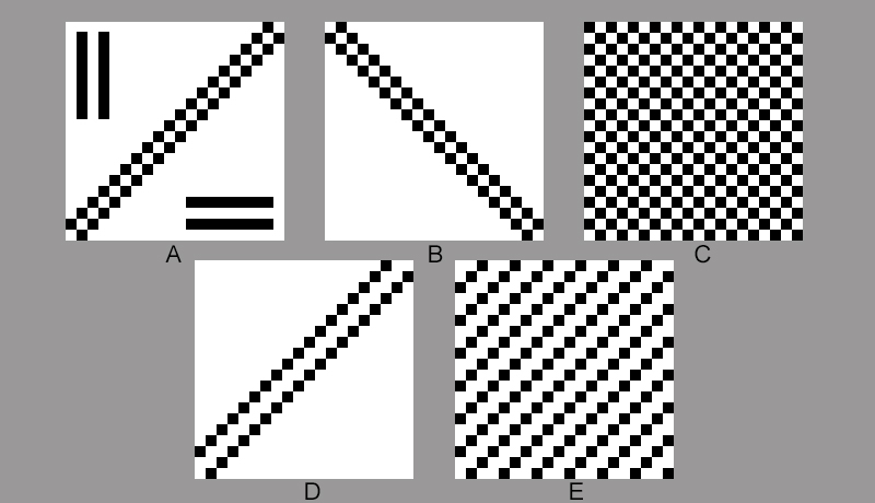

There is no question that non-aliased vertical or horizontal line-pairs at the Nyquist limit can be resolved on a raster-structured sensor or display. It can be fun to check what happens with patterns of 45° slanted non-aliased line pairs. In the above figure:

A - A one-pixel thick white line between two black lines of the same thickness, slanted clockwise. This is the Nyquist limit for a vertical or horizontal line pair. The shorter vertical and horizontal line sets are spaced at the same Nyquist limit.
B - The same lines as A, slanted counter-clockwise.
C - A pattern of multiple lines, same thickness and spacing as A and B. Are they slanted clockwise or counterclockwise?
D - A two-pixel thick white line between two one-pixel-thick black lines.
E - A pattern of slanted lines, same thickness and spacing as D. This is above the oblique Nyquist limit, so the direction of slant can be detected.

"Ideal" MTF of Micro 4/3

MTF (Modulation Transfer Function) measures how a system transfers the light modulation in a scene to the corresponding modulation in the recorded image. It is a combination of the modulation transfer functions across the chain of hardware and software stages, including the lens, sensor, ADC, demosaicing, firmware etc.

Although MTF is primarily used to evaluate how well an actual imaging system performs, it is very often used to evaluate lens performance. The general assumption, in this case, seems to be that the lens is the limiting factor in the hardware part of the chain, but this is not necessarily true. It is legitimate to ask, for example, what are the intrinsic limitations of a 20 Mpixel Micro 4/3 sensor. Ultimately, the discrete nature of pixels and of their values (8 bit for each color channel in JPG files) does pose limits to image resolution and MTF.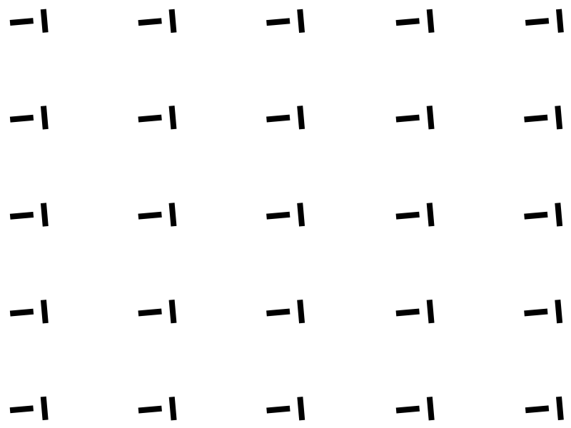

MTF is usually computed on an actual image recorded by a digital camera, often by a method using a resolution target type called slanted edge, which contains one or more sharp, slightly oblique borderlines between black and white areas. Since I was not interested in an actual MTF test of the whole camera system, I prepared a slanted edge target in Photoshop 2021 v. 22.4.3. This target has the same pixel count (5,185 x 3,888 pixels) as the OM-1 sensor. On a white background, I created a number of identical black slanted-edge rectangles, all tilted 5° counterclockwise (most software for measuring MTF works well with this, or a comparably small, inclination).

I generated this target as vector graphics in Photoshop, then exported it to 8-bit-per-channel JPG format using bicubic interpolation to smoothen the "jaggies" and saved the file at maximum JPG quality. The above figure shows an enlarged detail of a slanted edge, to show the effect of the interpolation. The tilted edge is particularly effective in MTF calculations because the transitions from black to white change in each successive line of pixels, so that the effects of aliasing can be averaged out.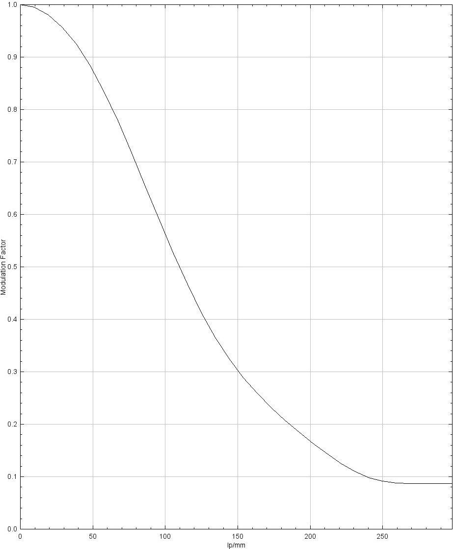

For measuring MTF, I used ImageJ by the NIH with the SE_MTF plugin by Carles Mitjà et al. The above MTF graph is one of the outputs generated by this plugin when one of the slanted edges in the target is selected. The graph is an average of the three color channels, which in this case are identical. It can be seen that the 50% MTF (0.5 on the y-axis) is located at approximately 115 lp/mm, which can be regarded as the maximum native theoretical resolution of this sensor at 50% MTF. A possible unknown is whether, and how much, sharpening is applied in-camera without telling the user. This would certainly alter the MTF. Demosaicing also likely affects MTF, but modern cameras lacking a physical anti-aliasing filter are getting better and better at avoiding artifacts while preserving as much image information as feasible.

The Nyquist limit, discussed above, in theory could allow a best-case resolution for vertical or horizontal line-pairs of

1,000 / 6.694 = 149 lp/mm

which is somewhat higher than the 50% MTF, but still quite close to it. In the case of line pairs slanted at 45°, the lp/mm resolution computed from the Nyquist limit is naturally lower, at 106.

The Nyquist limit for vertical/horizontal lines corresponds to an approximately 30% MTF as computed above. Below 30% MTF, the plotted results are only theoretical because one cannot resolve more than one line per pixel. However, even a line pattern below the Nyquist limit can in principle generate a non-zero amount of modulation, not as resolved line pairs, but as larger-scale moiré and/or other types of interference. (I make no claim that 30% MTF = Nyquist limit is a general rule. It just applies to this particular case.)

Conclusions

I collected or computed a few frequently-used parameters to use in calculations on Micro 4/3 cameras and their images, based on the OM System OM-1 sensor at full native resolution.